


前言
1、TensorFlow&Keras环境配置
这里选择Jupyter Notebook,好处不言而喻,可上网查看,这里不赘述;
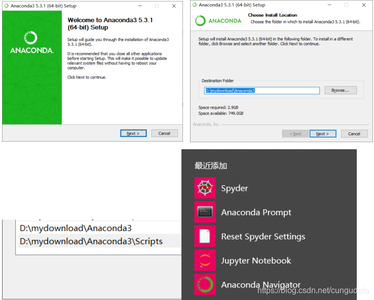
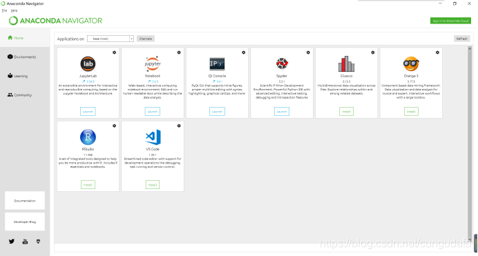
在windows10下安装Anaconda3并配置好环境,启动Anaconda Navigator,在其面板里下载配置TensorFlow、Keras、Jupyter Notebook、Vscode等库;
2、入门猫狗数据集实验
下载Kaggle狗猫数据集(mnist数据集略),按照 参考教程,完成狗猫数据集的分类实验;解释什么是overfit(过拟合),什么是数据增强?
3、理解卷积神经网络CNN
一、环境配置
1.安装anaconda
anaconda和python库是类似的,如果在同一计算机安装了两个环境,注意在IDE中选择对应的编译库。(pip安装都在anaconda目录下,而不在python安装目录下)
清华下载源:https://mirrors.tuna.tsinghua.edu.cn/anaconda/archive/
官方安装教程:http://docs.anaconda.com/anaconda/install/windows/
anaconda官方使用教程:
http://docs.anaconda.com/anaconda/user-guide/getting-started/
2.jupyter notebook配置
2.1修改运行时工作目录
jupyter默认打开的工作空间是C盘,当然,第一件事是修改工作目录了。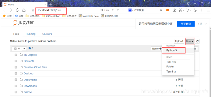
wn10直接打开菜单目录,修改快捷键的属性即可: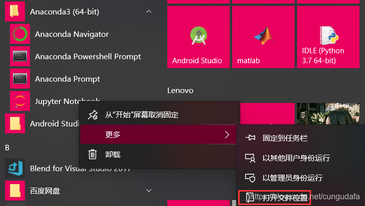
修改目标位置为你的工作空间(我的在D盘)和起始位置(置空):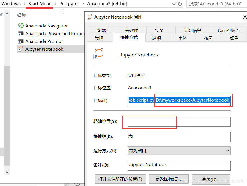
再打开jupyter,目录显示应该在你的指定位置。
jupyter是做数据处理和图像显示比任何一款IDE都优势一些的工具: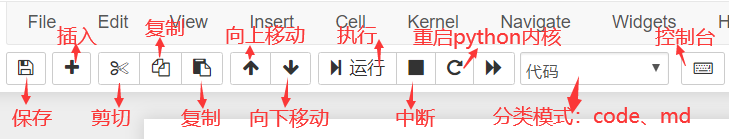
常用指令参考:https://blog.csdn.net/5hongbing/article/details/78526196
navigator使用教程:
http://docs.anaconda.com/anaconda/navigator/getting-started/
2.2添加jupyter_contrib_nbextensions插件
原生jupyter是没有:自动补全代码功能+pep8+字体大小+代码行号+拼写检查+目录索引这些功能的;当然有插件能帮我们完成.
安装jupyter_contrib_nbextensions库:
pip install jupyter_contrib_nbextensions -i https://pypi.douban.com/simple/配置到jupyter
jupyter contrib nbextension install --user --skip-running-check重启jupyter notebook
安装完成后,重新启动jupyter notebook,“Nbextensions”出现在导航栏中,勾选目录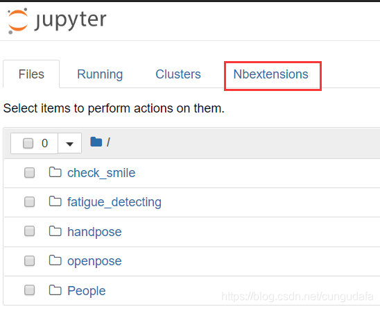
在原来的基础上勾选: “Table of Contents” 以及 “Hinterland”等,
(tips:autopep8需要安装pip install autopep8)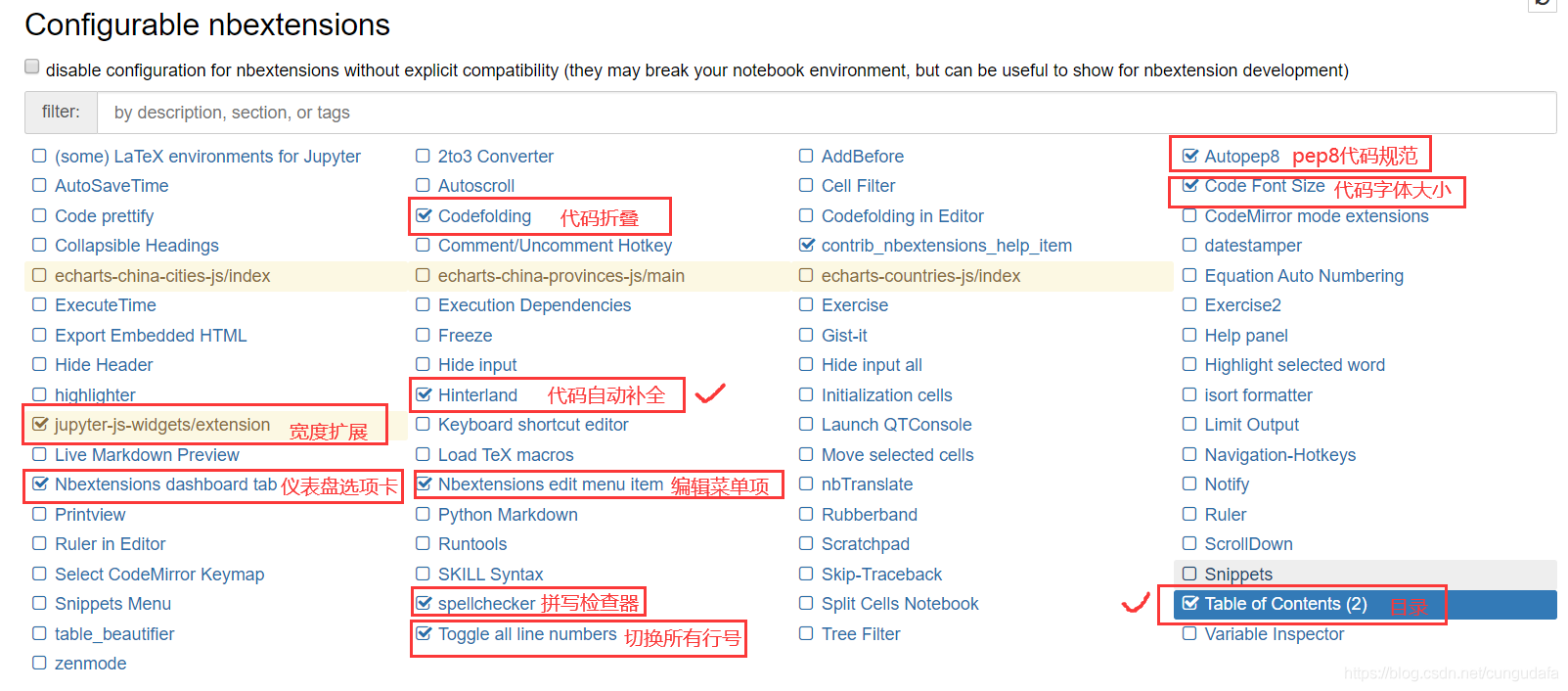
目录使用规则和Markdown相似,# 一级 ## 二级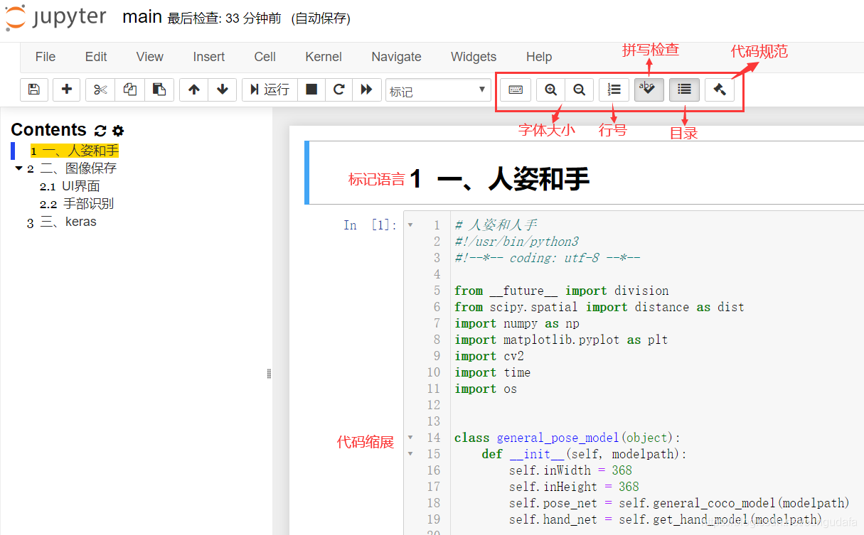
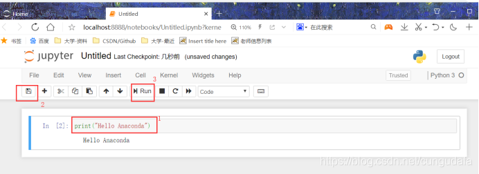
现在万事俱备了,接下来安装TensorFlow和keras。
3. 配置TensorFlow、Keras
有两种方法安装:
- 启动Anaconda Navigator,在其面板里下载配置TensorFlow、Keras
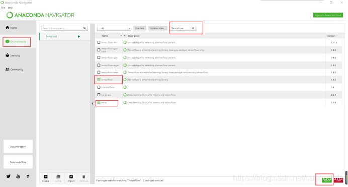
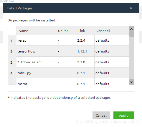
等待下载完成,测试: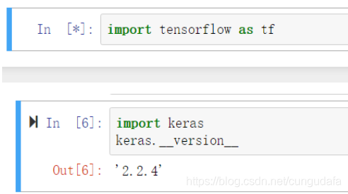
- 在cmd中pip安装:(第一种方法虽好,但我还是热衷于命令行🥰)
Files->New->Teminal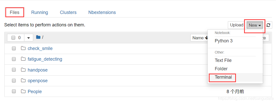
命令行安装:
exp:pip install tensorflow pip install keras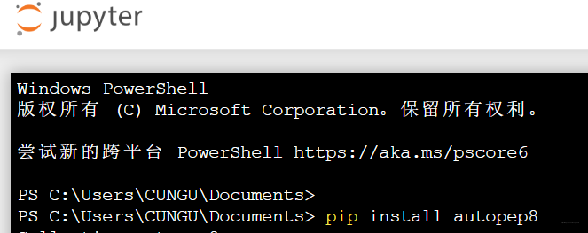
同理,在cmd中安装效果一样,肯定人和我的喜好一样,haha~
二、入门实例-猫狗数据集
1.制作数据集
在数据分析处理这一块,原数据模型是最值价的了,常用的是kaggle网站的数据集
- 从Kaggle下载猫狗数据集
或者:链接:https://pan.baidu.com/s/13hw4LK8ihR6-6-8mpjLKDA 密码:dmp4- 根据教程完成对猫狗数据集的处理:
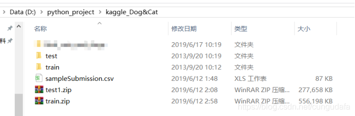
(1)运行程序:根据命名对图片分类: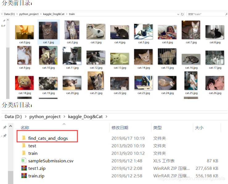
详细文件内容: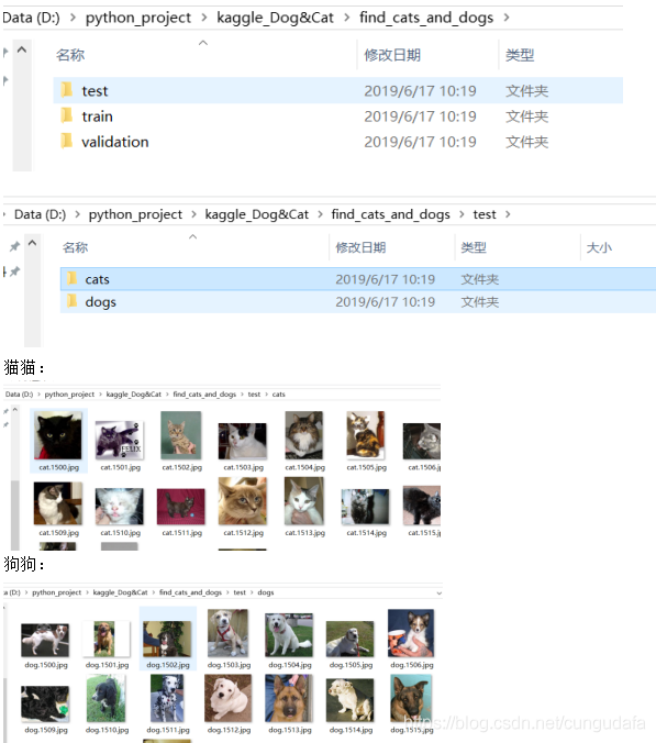
图片分类:
import os, shutil
# The path to the directory where the original
# dataset was uncompressed
original_dataset_dir = 'D:/python_project/kaggle_Dog&Cat/train'

# The directory where we will
# store our smaller dataset
base_dir = 'D:/python_project/kaggle_Dog&Cat/find_cats_and_dogs'
os.mkdir(base_dir)

# Directories for our training,
# validation and test splits
train_dir = os.path.join(base_dir, 'train')
os.mkdir(train_dir)
validation_dir = os.path.join(base_dir, 'validation')
os.mkdir(validation_dir)
test_dir = os.path.join(base_dir, 'test')
os.mkdir(test_dir)

# Directory with our training cat pictures
train_cats_dir = os.path.join(train_dir, 'cats')
os.mkdir(train_cats_dir)

# Directory with our training dog pictures
train_dogs_dir = os.path.join(train_dir, 'dogs')
os.mkdir(train_dogs_dir)

# Directory with our validation cat pictures
validation_cats_dir = os.path.join(validation_dir, 'cats')
os.mkdir(validation_cats_dir)

# Directory with our validation dog pictures
validation_dogs_dir = os.path.join(validation_dir, 'dogs')
os.mkdir(validation_dogs_dir)

# Directory with our validation cat pictures
test_cats_dir = os.path.join(test_dir, 'cats')
os.mkdir(test_cats_dir)

# Directory with our validation dog pictures
test_dogs_dir = os.path.join(test_dir, 'dogs')
os.mkdir(test_dogs_dir)

# Copy first 1000 cat images to train_cats_dir
fnames = ['cat.{}.jpg'.format(i) for i in range(1000)]
for fname in fnames:
    src = os.path.join(original_dataset_dir, fname)
    dst = os.path.join(train_cats_dir, fname)
    shutil.copyfile(src, dst)

# Copy next 500 cat images to validation_cats_dir
fnames = ['cat.{}.jpg'.format(i) for i in range(1000, 1500)]
for fname in fnames:
    src = os.path.join(original_dataset_dir, fname)
    dst = os.path.join(validation_cats_dir, fname)
    shutil.copyfile(src, dst)

# Copy next 500 cat images to test_cats_dir
fnames = ['cat.{}.jpg'.format(i) for i in range(1500, 2000)]
for fname in fnames:
    src = os.path.join(original_dataset_dir, fname)
    dst = os.path.join(test_cats_dir, fname)
    shutil.copyfile(src, dst)

# Copy first 1000 dog images to train_dogs_dir
fnames = ['dog.{}.jpg'.format(i) for i in range(1000)]
for fname in fnames:
    src = os.path.join(original_dataset_dir, fname)
    dst = os.path.join(train_dogs_dir, fname)
    shutil.copyfile(src, dst)

# Copy next 500 dog images to validation_dogs_dir
fnames = ['dog.{}.jpg'.format(i) for i in range(1000, 1500)]
for fname in fnames:
    src = os.path.join(original_dataset_dir, fname)
    dst = os.path.join(validation_dogs_dir, fname)
    shutil.copyfile(src, dst)

# Copy next 500 dog images to test_dogs_dir
fnames = ['dog.{}.jpg'.format(i) for i in range(1500, 2000)]
for fname in fnames:
    src = os.path.join(original_dataset_dir, fname)
    dst = os.path.join(test_dogs_dir, fname)
    shutil.copyfile(src, dst)
(2)统计图片数量:
print('total training cat images:', len(os.listdir(train_cats_dir)))
print('total training dog images:', len(os.listdir(train_dogs_dir)))
print('total validation cat images:', len(os.listdir(validation_cats_dir)))
print('total validation dog images:', len(os.listdir(validation_dogs_dir)))
print('total test cat images:', len(os.listdir(test_cats_dir)))
print('total test dog images:', len(os.listdir(test_dogs_dir)))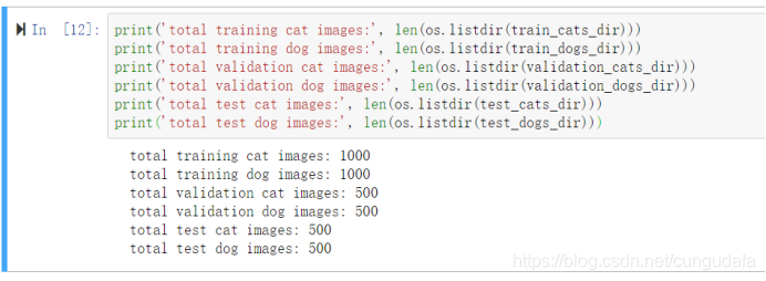
猫狗训练图片各1000张,验证图片各500张,测试图片各500张。
2.卷积神经网络CNN
快速开发基准模型:面对一个任务,通常需要快速验证想法,并不断迭代。因此开发基准模型通常需要快速,模型能跑起来,效果比随机猜测好一些就行,不用太在意细节。至于正则化、图像增强、参数选取等操作,后续会根据需要来进行。^3
2.1 网络模型搭建
model.summary()输出模型各层的参数状况
from keras import layers
from keras import models

model = models.Sequential()
model.add(layers.Conv2D(32, (3, 3), activation='relu',
                        input_shape=(150, 150, 3)))
model.add(layers.MaxPooling2D((2, 2)))
model.add(layers.Conv2D(64, (3, 3), activation='relu'))
model.add(layers.MaxPooling2D((2, 2)))
model.add(layers.Conv2D(128, (3, 3), activation='relu'))
model.add(layers.MaxPooling2D((2, 2)))
model.add(layers.Conv2D(128, (3, 3), activation='relu'))
model.add(layers.MaxPooling2D((2, 2)))
model.add(layers.Flatten())
model.add(layers.Dense(512, activation='relu'))
model.add(layers.Dense(1, activation='sigmoid'))
model.summary()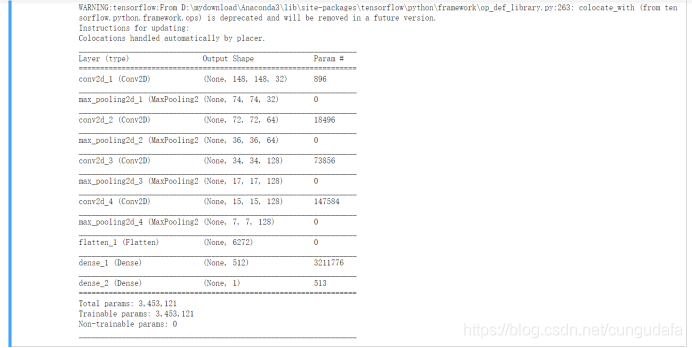
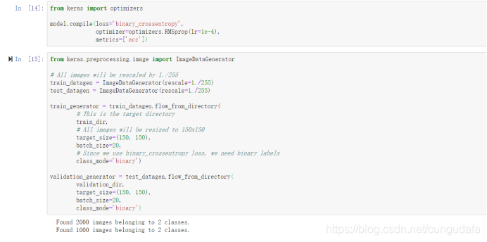
2.2 图像生成器读取文件中数据
model.compile()优化器(loss:计算损失,这里用的是交叉熵损失,metrics: 列表,包含评估模型在训练和测试时的性能的指标)- 所有图片(2000张)重设尺寸大小为150x150大小
- ImageDataGenerator就像一个把文件中图像转换成所需格式的转接头,通常先定制一个转接头train_datagen,它可以根据需要对图像进行各种变换,然后再把它怼到文件中(flow方法是怼到array中),约定好出来数据的格式(比如图像的大小、每次出来多少样本、样本标签的格式等等)。这里出来的train_generator是个(X,y)元组,X的shape为(20,150,150,3),y的shape为(20,)
2.3 开始训练
generator()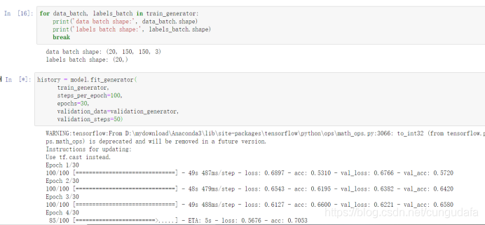
loss 损失函数值,与你定义的损失函数值相关
acc 准确率
mean_absolute_error 平均绝对误差
前面带val_表示你的模型在验证集上进行验证时输出的这三个值,验证在每个epoch后进行
一个选拔的故事(acc,loss,val_acc,val_loss的区别):
http://www.pianshen.com/article/5415291383/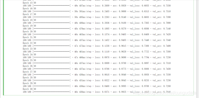
2.4 保存模型
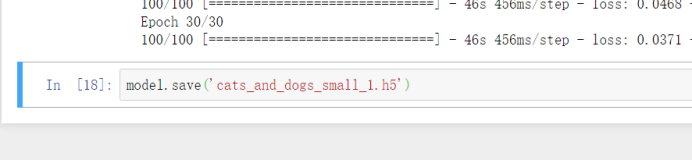
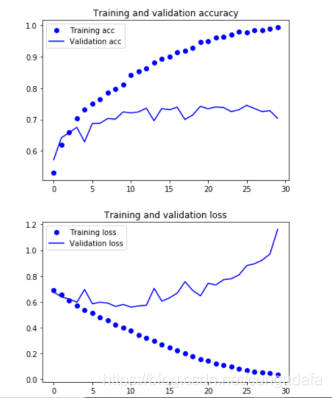
2.5 结果可视化
训练结果如下图所示,很明显模型上来就过拟合了,主要原因是数据不够,或者说相对于数据量,模型过复杂(训练损失在第30个epoch就降为0了)。import matplotlib.pyplot as plt
acc = history.history[‘acc’]
val_acc = history.history[‘val_acc’]
loss = history.history[‘loss’]
val_loss = history.history[‘val_loss’]
epochs = range(len(acc))
plt.plot(epochs, acc, ‘bo’, label=’Training acc’)
plt.plot(epochs, val_acc, ‘b’, label=’Validation acc’)
plt.title(‘Training and validation accuracy’)
plt.legend()
plt.figure()
plt.plot(epochs, loss, ‘bo’, label=’Training loss’)
plt.plot(epochs, val_loss, ‘b’, label=’Validation loss’)
plt.title(‘Training and validation loss’)
plt.legend()
plt.show()
## 3.根据基准模型进行调整
为了解决过拟合问题,可以减小模型复杂度,也可以用一系列手段去对冲,比如增加数据(图像增强、人工合成或者多搜集真实数据)、L1/L2正则化、dropout正则化等。这里主要介绍CV中最常用的图像增强。
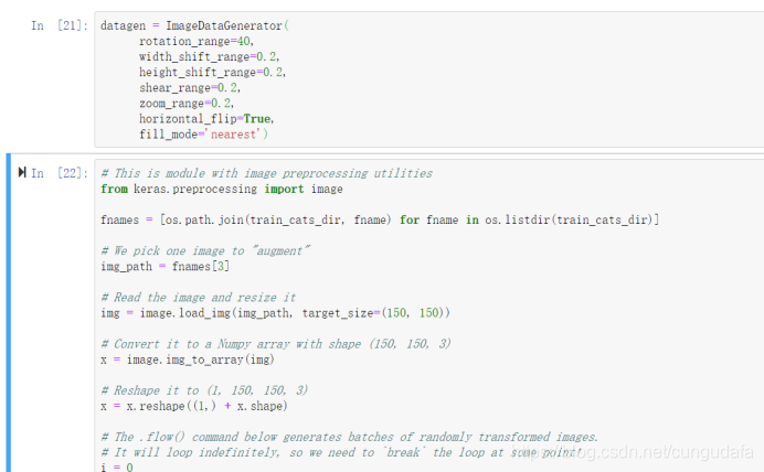
### 3.1 图像增强方法
在Keras中,可以利用图像生成器很方便地定义一些常见的图像变换。将变换后的图像送入训练之前,可以按变换方法逐个看看变换的效果。代码如下:

```python
datagen = ImageDataGenerator(
rotation_range=40,
width_shift_range=0.2,
height_shift_range=0.2,
shear_range=0.2,
zoom_range=0.2,
horizontal_flip=True,
fill_mode='nearest')
# This is module with image preprocessing utilities
from keras.preprocessing import image
fnames = [os.path.join(train_cats_dir, fname) for fname in os.listdir(train_cats_dir)]
# We pick one image to "augment"
img_path = fnames[3]
# Read the image and resize it
img = image.load_img(img_path, target_size=(150, 150))
# Convert it to a Numpy array with shape (150, 150, 3)
x = image.img_to_array(img)
# Reshape it to (1, 150, 150, 3)
x = x.reshape((1,) + x.shape)
# The .flow() command below generates batches of randomly transformed images.
# It will loop indefinitely, so we need to `break` the loop at some point!
i = 0
for batch in datagen.flow(x, batch_size=1):
plt.figure(i)
imgplot = plt.imshow(image.array_to_img(batch[0]))
i += 1
if i % 4 == 0:
break
plt.show()3.2 模型调整
- 将这几种选定的图像增强方法添加进训练集的生成器中(train_datagen);
- 在模型结构中加入一层Dropout(在Flatten层后加上 Dropout(0.5))。
调整并重新训练改为100个epoch。重新训练后的结果如图所示。可以看出,准确率由基准的67%提高到82%,进一步调整模型还可以提升到86%左右。但是进一步就再难以继续提升了,因为数据太少,且模型比较粗糙,下一节我们会采取其他更有效的措施。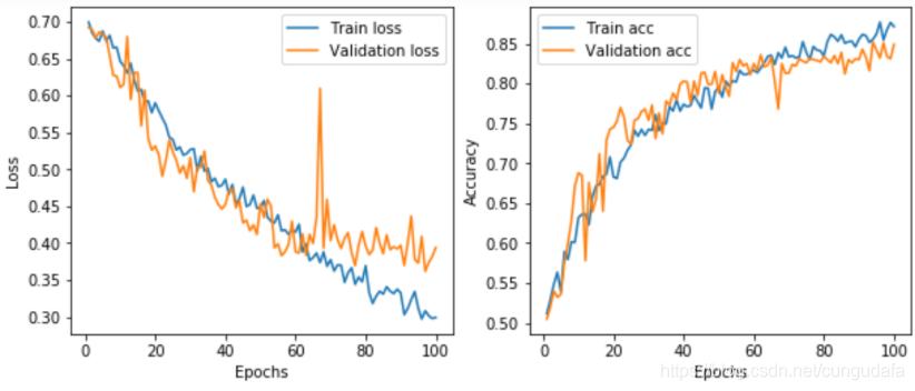
4. 卷积神经网络的可视化
导入100次训练模型,查看模型参数
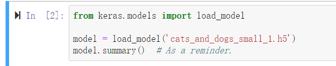
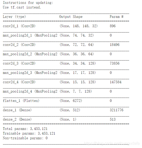
 from keras.models import load_model
 model = load_model('cats_and_dogs_small_1.h5')
 model.summary()  # As a reminder.
模型预处理
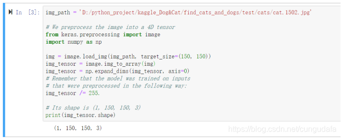
 img_path = 'D:/python_project/kaggle_Dog&Cat/find_cats_and_dogs/test/cats/cat.1502.jpg'

 # We preprocess the image into a 4D tensor
 from keras.preprocessing import image
 import numpy as np

 img = image.load_img(img_path, target_size=(150, 150))
 img_tensor = image.img_to_array(img)
 img_tensor = np.expand_dims(img_tensor, axis=0)
 # Remember that the model was trained on inputs
 # that were preprocessed in the following way:
 img_tensor /= 255.

 # Its shape is (1, 150, 150, 3)
 print(img_tensor.shape)
输入一张不属于网络的猫的图像
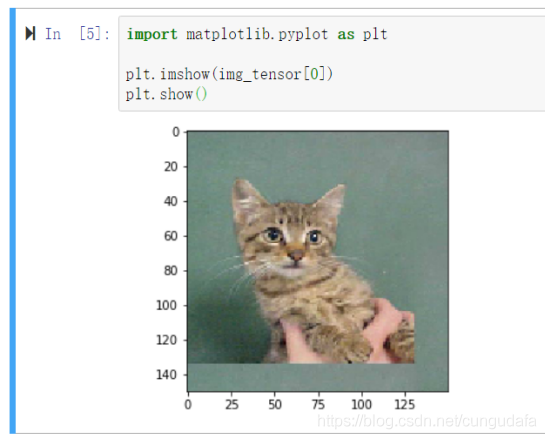
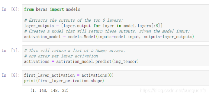
 import matplotlib.pyplot as plt

 plt.imshow(img_tensor[0])
 plt.show()
为了提取想要查看的特征图,我们需要创建一个Keras模型,以图像批量作为输入,并输出所有卷积层和池化层的激活。为此,我们需要使用Keras的Model类。模型实例化需要两个参数:一个输入张量(或输入张量的列表)和一个输出张量(或输出张量的列表)。
layer_outputs:提取前8层的输出
activation_model:创建一个模型,给定模型的输入,可以返回这些输出
activations :输入一张图像,这个模型将返回8个Numpy数组组成的列表,每个层激活对应一个Numpy数组
它是大小为148*148的特征图,有32个通道。我们来绘制原始模型第3个通道: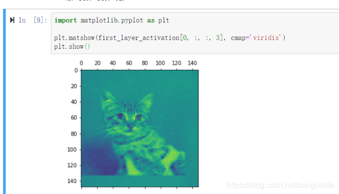
再看看第30个通道: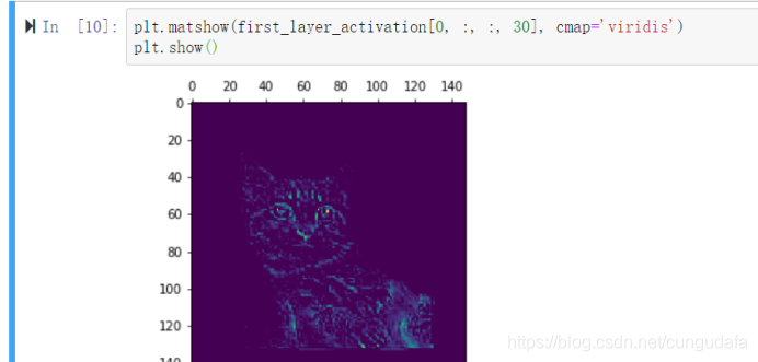
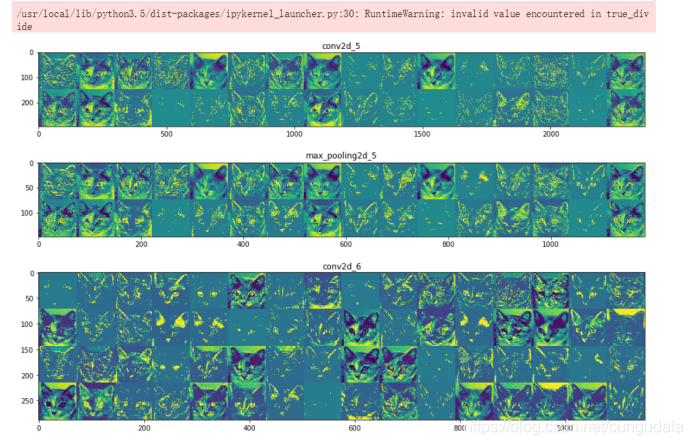
我们可以看到,似乎不同通道对于图像检测有不同侧重,比如第3个通道更侧重于边缘检测,第30个通道更侧于”绿色圆点“检测。下面我们来绘制网络中所有激活的完整可视化图。我们需要在8个特征图里的每一个都提取并绘制一个通道,然后将结果叠加在一个大的图像张量中,按通道并排。
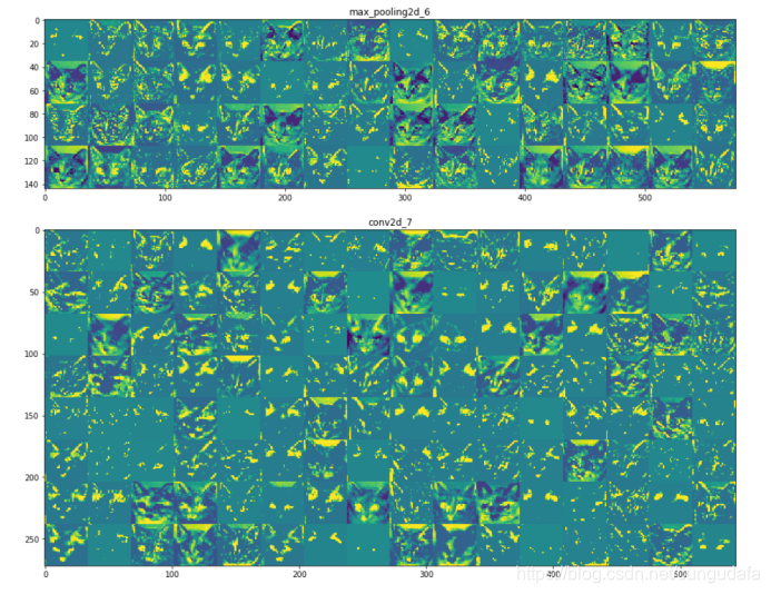
三、CNN模型
3.1 神经网络结构
- 单层神经网络
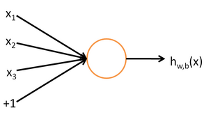
表达式:(也称为Logistic回归模型)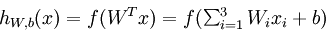
- 多层神经网络结构
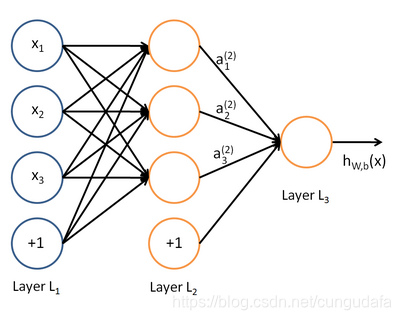
表达式:(如此一层一层的加上去,最终就形成了深度神经网络)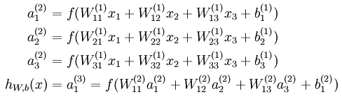
3.2 卷积神经网络CNN
参考:cnn算法
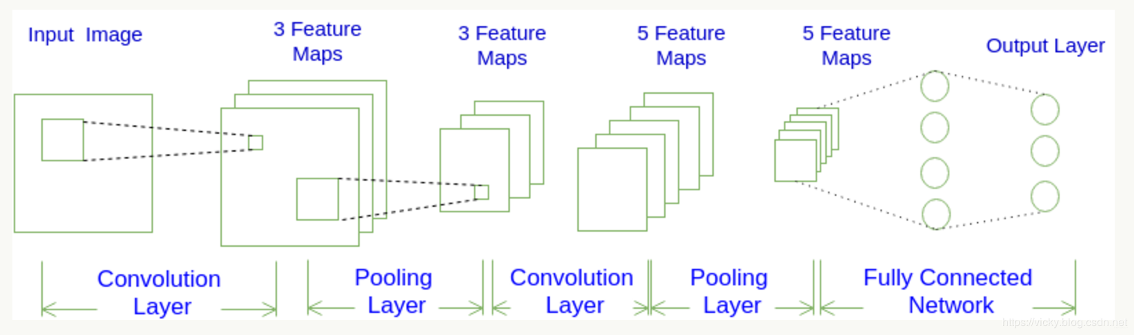
卷积神经网络CNN的结构一般包含这几个层:^1
- 输入层:用于数据的输入
- 卷积层:使用卷积核进行特征提取和特征映射
- 激励层:由于卷积也是一种线性运算,因此需要增加非线性映射
- 池化层:进行下采样,对特征图稀疏处理,减少数据运算量。
- 全连接层:通常在CNN的尾部进行重新拟合,减少特征信息的损失
CNN的三个特点:
- 局部连接:这个是最容易想到的,每个神经元不再和上一层的所有神经元相连,而只和一小部分神经元相连。这样就减少了很多参数
- 权值共享:一组连接可以共享同一个权重,而不是每个连接有一个不同的权重,这样又减少了很多参数。
- 下采样:可以使用Pooling来减少每层的样本数,进一步减少参数数量,同时还可以提升模型的鲁棒性。